
How to Build Your First Machine Learning Model Step by Step
Master Guide 2025
The process of creating your first machine learning model can be a daunting task however with proper instructions and an organized approach you will be able to build an effective predictive model in several hours. This step by step tutorial guides you through the whole model learning process starting beginning with the fundamentals and the deployment of your model.
It doesnt matter if youre a software engineer moving into data science an executive trying to harness artificial intelligence or student looking to explore the possibilities of machine learning the tutorial is designed to provide an in depth practical understanding. Learn the most important techniques including the preprocessing of data feature engineering modeling model selection as well as hyperparameter tuning and assessment of performance with industry standard frameworks and tools.
At the conclusion of this tutorial youll have created a full machine learning system using Python programming the scikit learn library and pandas to manipulate data. In addition youll be able to comprehend the basic workflow data experts and machine learning engineers use in real world applications that span industries such as finance healthcare ecommerce and even technology.
Read Also – The Role of Machine Learning in Predictive Analytics for Businesses: Master Guide 2025
Understanding Machine Learning Fundamentals
What is Machine Learning?
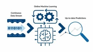
Machine learning is a type of artificial intelligence which enables computer systems to discover patterns in data with no explicitly programming. Instead of manually writing down rules algorithms find connections between the input and output objectives through statistical analysis and mathematical optimization.
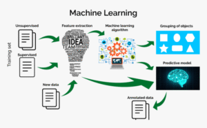
The process of machine learning involves putting training data to algorithms which identify patterns correlations and structure. The patterns that are learned allow models to predict new undiscovered information. Supervised learning makes use of labeled examples Unsupervised learning uncovers the hidden structure while reinforcement learning is a process of trials and errors.
Types of Machine Learning Problems
Classification assigns data points to classes or categories that are distinct. Binary classification is a way of distinguishing between two results like spam versus legitimate mail and multi class classification addresses multiple categories such for identifying species of animals or the types of product.
Regression predicts continuous numerical value. Its applications include predicting house prices as well as temperature forecasting estimates of sales as well as analyses of the stock market. Regression models generate data on a continuous scale instead of distinct categories.
Clustering clusters similar data points with no predefined label. Document organization customer segmentation and the detection of anomalies rely on the clustering algorithm. This method of learning that is unsupervised reveals the natural patterns of data groupings.
Essential Machine Learning Terminology
Knowing the key terms will speed up your journey to learning. Features define input variables or the attributes that define every single data item. labels or targets represent outcomes you need to be able to predict. Data for training will teach you the model as testing data examines the models performance using untested scenarios.
Overfitting happens when models remember the training data instead of making generalized patterns. Underfitting occurs in models that arent able to comprehend the complexity of data. Hyperparameters can be defined as settings for configuration that regulate the learning process. They are different from the model parameters that are obtained from information.
Accuracy evaluates overall accuracy While accuracy as well as recall assess the effectiveness of particular categories. Cross validation tests the models reliability through conducting tests and training on various datasets. Knowing these principles is essential to build effective machine learning solutions.
Setting Up Your Development Environment
Installing Python and Essential Libraries
Python is now the most popular programming language in machine learning thanks to its ease of use the abundance of libraries and extensive support from the community. Install Python 3.8 or greater by visiting python.org. A lot of developers use the Anaconda distribution that comes with the essential data science tools that are pre configured.
The most important libraries to your machine learning toolkit comprise NumPy to perform numerical computation as well as array operation Pandas for data manipulation and analysis Scikit Learn for machine learning tools and algorithms Matplotlib and Seaborn for visualization of data and Jupyter Notebook to allow interactive programming.
Install the libraries by using the pip Package Manager: Pip install Numpy Pandas scikit learn matplotlib seaborn jupyter. If you are working on deep learning further frameworks like TensorFlow Keras or PyTorch are required but well concentrate on conventional machine learning to create your first design.
Choosing the Right Development Tools
Jupyter Notebook is an interactive platform that is ideal for exploration and learning. Code cells operate independently which allows for iterative development as well as immediate feedback. Markdown cells permit documentation in conjunction with codes resulting in self contained instructional videos.
The VS Code that comes with Python extensions is a complete integrated development environment to produce code. PyCharm is a specific Python development tools that have excellent ability to debug. Google Colab is a no cost Jupyter notebooks that run on the cloud that include GPU access. It eliminates the need for local setup.
Pick tools that fit your preferred workflows and needs. For beginners it is common to start with Jupyter Notebook to gain experience before moving to IDEs for more complex project. Cloud platforms such as Colab provide access to a wider audience and require just a browser on the internet.
Step 1: Defining Your Problem and Objectives
Choosing Your First Project
Begin with a clearly defined challenge and easily accessible data. Some popular beginner projects are forecasting the cost of a house (regression) or classifying Iris flower species (classification) as well as recognising handwritten digits (image classification) as well as predicting the likelihood of customers the rate of churn (binary classification).
The Iris data Boston housing prices MNIST numbers and Titanic survival statistics are excellent start data points. Clean well documented data let you focus on the machine learning process and avoid the hassle of navigating messy information at first.
Select problems that truly interest you. The motivation of learning is a key factor in overcoming challenges. Practical applications such as predicating diabetes risk analysing film reviews or predicting stock market trends offer stimulating contexts for teaching the fundamental methods.
Defining Success Metrics
A clear set of success criteria guides model design and assessment. When it comes to classification accuracy measures how accurate the predictions are. But accuracy can be misleading due to uneven data where one type of class has the upper hand.
Precision shows what percentage of predictions that were positive in fact correct. Recall determines the percentage of real positives could be correctly identified. F1 score weighs recall and precision by providing one metric that can be used to evaluate the model.
For regression problems mean squared error (MSE) penalizes large errors heavily. The root mean squared error (RMSE) returns error in its original units which improves understanding. The mean absolute error (MAE) treats all errors equally. R squared determines the share of variation explained in the framework.
Step 2: Data Collection and Exploration
Finding and Loading Datasets
High quality data constitutes the base of effective machine learning models. Public repositories such as Kaggle UCI Machine Learning Repository Google Dataset Search as well as AWS Open Data Registry provide millions of datasets that are free and available across a range of domains.
If you are starting out with your first project you can use the built in scikit learn data sets that are accessible via sklearn.datasets. The iris classification dataset can be loaded: from sklearn.datasets import load_iris. iris = load_iris(). It returns targets features as well as descriptions in a convenient package.
CSV files are the standard file format used for data. Pandas reads CSV data easily: import pandas as pd; df = pd.read_csv(data.csv). Discover various formats including Excel file formats JSON SQL databases Web APIs and SQL databases. Skills in data engineering are becoming increasingly essential for the actual work.
Exploratory Data Analysis (EDA)
Analyzing your data with EDA can prevent costly errors and provides insight. Beginning by examining the basics of statistical data with df.describe() that displays counts means standard deviation minimal maximal quartiles and maximum in numerical data.
Examine data types using df.dtypes and identify any missing values with df.isnull().sum(). The missing data needs special attention by imputation or elimination. Knowing the distribution of data in relation to outliers distributions and the relationship between variables can help make preprocessing decisions.
Visualization highlights patterns that cannot be seen from raw numbers. Histograms display the distribution of features. Box graphs highlight the outliers. Scatter plots reveal relationships between variables. Correlation matrixes that are displayed as heatmaps the interactions between variables. Seaborn helps create stunning insightful visualizations.
Categorical functions require encryption prior to the model is trained. Examine unique values using df[column].unique() and value counts with df[column].value_counts(). Learning about class balance when defining class targets helps to avoid biases towards major groups.
Step 3: Data Preprocessing and Feature Engineering
Handling Missing Values
The real world data often contain data that is missing due to a variety of reasons like collection error and system malfunctions or deliberate omissions. Find patterns of missing data to select the most appropriate methods for handling.
Elimination Eliminates columns and rows that have missing values. df.dropna() removes rows that contain value that is null. This method is simple and works well when there is a small amount of missing data and its random. But frequent deletion decreases sampling size and could cause bias.
Imputation replaces the missing value with estimations. Simple strategies include using mean median or mode for numerical features: df[column].fillna(df[column].mean()). When it comes to categorical characteristics you should use the most frequently used type of category. Modern techniques such as K nearest neighbor Imputation take into account relationships between the characteristics.
Feature Scaling and Normalization
Machine learning algorithms work better when the features are operating on comparable scales. Standardization transforms features to have zero mean and unit variance using StandardScaler: from sklearn.preprocessing import StandardScaler; scaler = StandardScaler(); X_scaled = scaler.fit_transform(X).
Min max Normalization is a method of scaling features within an undefined range usually between 0 and 1 with the help of MinMaxScaler. It preserves zero values and is beneficial for neural networks. Distance based algorithms such as k nearest neighbor and support vector machines in particular benefit from the scaling.
Tree based algorithms including decision trees random forest and gradient boost remain agnostic with regard to scaling. But standardizing data seldom harms and in many cases helps and is a great routine.
Encoding Categorical Variables
Machine learning models need the input of numbers requiring categorical feature encoders. One hot Encoding generates binaries for every class employing pd.get_dummies() or OneHotEncoder. Every observation is given 1 point within its column of category while the other columns get 0.
For categories that have natural order such as “low medium high” the encoder for labels assigns integers preserving the an order. Use scikit learns LabelEncoder or pandas mapping: df[size].map().
The high cardinality characteristics with a variety of unique value create excessive columns via one hot encoders. Think about the use of target decoding frequency encoding or classifying distinct types. Be sure to balance expressiveness and dimensionality in order so as to not create feature spaces with a lot of features.
Feature Engineering and Selection
Making informative features using available data usually improves the performance of models better than choosing an algorithm. Domain specific knowledge is a guide to feature design. To create date columns you must extract days of the week months or quarter. Also you can include holiday dates. Combining features using division multiplication or polynomial expressions to show interactions.
Features choice determines the most reliable variables and reduces dimensionality as well as duration of training. Filtering methods employ methods of statistical testing such as the mutual or correlation test. Methods like wrapper Recursive feature elimination analyze specific subsets by training models. Methods that are embedded such as Lasso regression make selections in the course of the training.
Try all the features that are available to build your model and then play around with features in case performance isnt as high or training difficult or slow. Feature engineering is a process that requires imagination and know how in the field developed by practice and experiments.
Step 4: Dividing the data into Testing and Training Sets
Understanding Train Test Split
Dont test models using the same information used in learning. Models are taught to recall training exercises which produce unrealistic performances estimates. The split between the train and test is used to reserve information for impartial analysis mimicking real world scenarios when models are exposed to new information.
It is common practice to allocate 70 to 80% of the data used for learning and 20 30% to testing. Use scikit learns train_test_split: from sklearn.model_selection import train_test_split; X_train X_test y_train y_test = train_test_split(X y test_size=0.2 random_state=42).
Random_state parameter ensures consistency. random_state parameter assures consistency through fixing the split in random. This allows for an accurate comparison between various models and parameters. The stratified splitting method with stratify=y ensures that class percentages are maintained for both sets. This is vital to avoid classification imbalances.
Cross Validation for Robust Evaluation
Simple splits in training and testing can yield diverse results based on what data samples are included in the collection. Cross validation tackles this problem by continually studying and testing different datasets and aggregating results to provide reliable performance estimations.
K fold cross validation divides data into k equal parts. The model is trained on folds k 1 and test the other fold repeatedly every fold acting as a testing set for one time. Five or ten folds can be the most common options for balancing computations and variation reduction.
Implement cross validation using cross_val_score: from sklearn.model_selection import cross_val_score; scores = cross_val_score(model X_train y_train cv=5). The result is figures of performance per fold and allows the calculation of mean accuracy as well as the standard deviation.
Step 5: Selecting and Training Your First Model
Choosing the Right Algorithm
The algorithm selection is based on the problem nature the datas characteristics and the performance demands. If you are starting your first project in classification logistic regression provides a straightforward but effective starting point. Contrary to its name logistic regression is a method of classification that relies on probabilistic prediction.
Decision trees are interpretable models which show the exact way that predictions are created by branches. Random forests mix several decision trees increasing the accuracy of predictions and decreasing overfitting by the process of ensemble learning. Vector machines that support are ideal in smaller databases with clear separation between classes.
To solve regression issues begin by using the linear model for establishing the base. Ridge regression and Lasso regression include regularization in order to avoid the overfitting. Random forest Regressors and gradient boosting machines are able to handle non linear relationships efficiently.
Training Your Model
Learning a model in scikit learn takes only a few pages of. Incorporate the chosen algorithm From sklearn.linear_model the import of LogisticRegression. Initialize the model: model = LogisticRegression(). Make the model fit to the information from the training process: model.fit(X_train y_train).
The fitting method does the actual learning process by adjusting the parameters for the model in order to limit mistakes in the prediction of training data. The process is different for each algorithm. Logistic regression employs maxima likelihood estimation while neural networks utilize the gradient descent algorithm.
Training times vary based on the data dimension size of the feature as well as the algorithms complexity. Simple models can train in mere minutes on smaller datasets but deep learning models might take days or even hours to train to train large databases using GPUs.
Making Predictions
After training generate predictions on test data: y_pred = model.predict(X_test). In order to classify the data this produces the predicted labels for classes. Numerous algorithms provide probabilities estimates using prediction_proba() useful to make decisions based on confidence.
Compare the predictions with real labels to determine the your performance. Analyze results with confusion matrices to classify or scatter plots to compare predictions with actual data to determine regression.
Step 6: Evaluating Model Performance
Classification Metrics
Accuracy calculates the percentage of correct predictions: from sklearn.metrics import accuracy_score; accuracy = accuracy_score(y_test y_pred). Although it is intuitive accuracy can be misleading on imbalanced datasets where most classes is accurate without having learned any meaningful.
The confusion matrix shows true positives true negatives false positives and false negatives: from sklearn.metrics import confusion_matrix; cm = confusion_matrix(y_test y_pred). The matrix shows which classes it confuses as well as guiding the improvement.
Precision determines the accuracy of positive predictions: precision = (TP + FP). (TP + FP). Recall or sensitivity is a measure of the completeness of positive detection. It is measured by recall is TP / (TP + FN). F1 score harmonically blends recall and precision and balances both of them.
Curves of ROC depict true positive rate against false positive rate over various thresholds for classification. AUC (area under the curve) sums up ROC results in one number with 1.0 is a perfect representation of classification.
Regression Metrics
Mean Absolute Error (MAE) averages the absolute differences between predictions and actual values: from sklearn.metrics import mean_absolute_error; mae = mean_absolute_error(y_test y_pred). MAE uses similar units as the variable of interest which makes it a readable.
Mean Squared Error (MSE) squares errors before averaging heavily penalizing large mistakes: from sklearn.metrics import mean_squared_error; mse = mean_squared_error(y_test y_pred). Root Mean Squared Error (RMSE) takes the square root of MSE and then returns to the their original units.
R squared determines the amount of variance within the variables that is explained through the models. The range of values is from 0 to 1. Higher numbers indicating better fitting. Positive R squared is a sign that models do less well than they can predict the median.
Step 7: Improving Model Performance
Hyperparameter Tuning
Hyperparameters influence algorithmic behavior but dont learn by the data. Examples include the depth of trees within decision trees regularization intensity for linear models and the number of neighbors within a KNN. The optimal hyperparameters for a given dataset vary.
Grid search exhaustively tries all combinations from predefined parameter grids: from sklearn.model_selection import GridSearchCV; param_grid = ; grid_search = GridSearchCV(model param_grid cv=5); grid_search.fit(X_train y_train).
Random Search tests parameter combinations in random fashion usually locating good solutions quicker than grid searches to search for spaces with high dimensions. Bayesian Optimization efficiently analyzes the parameter space on the basis of previous results providing the most efficient way to approach.
Handling Overfitting and Underfitting
Overfitting happens when models do very well with training data however they perform poorly with testing data suggesting that the model is learning rather than memorizing. Strategies to stop overfitting are cutting down on model complexity implementing regularization gathering more data for training as well as using cross validation.
Regularization penalizes complicated models by introducing terms into the loss function. Regularization of L1 (Lasso) causes certain coefficients to zero while allowing the feature selection. Regularization of L2 (Ridge) decreases coefficients towards zero but doesnt eliminate them.
Dropout randomly deactivates neurons during neural network training preventing co adaptation. Initial stoppage evaluates the performance of validation during the training process and stops when performance declines. Data enhancement artificially broadens the set of training via transformations.
Insufficient fitting of models indicates they arent simple to be able to detect patterns in data. Options include increasing the models complexity by adding new features decreasing regularization or attempting more advanced methods. Be aware of the risk of overfitting.
Step 8: Deploying Your Model
Saving and Loading Models
Store models that have been trained on disk so that they can be used again without needing to learn: import joblib; joblib.dump(model model.pkl). The serialization will preserve all the learned parameters and settings. Load models later: model = joblib.load(model.pkl).
In the case of deep learning models TensorFlow and PyTorch have specialized saving tools for that preserve the architecture and weights. Control the version of your model along with your code and track parameters performance and details about training.
Creating a Simple Prediction Interface
Web based applications allow non technical users to connect to the model. Flask and FastAPI develop REST APIs that accept the input information and delivering the predictions. An example Flask application:
Python
from flask import Flask request jsonify import joblib app = Flask(__name__) model = joblib.load(model.pkl) @app.route(/predict methods=[POST]) def predict(): data = request.get_json() prediction = model.predict([data[features]]) return jsonify()
Streamlit provides even more simple deployment to data science related applications by allowing the creation of interactive web applications using a minimum of programming. Cloud based platforms such as AWS SageMaker Google Cloud AI Platform and Azure ML are an automated deployment infrastructure.
Best Practices and Common Pitfalls
Data Leakage Prevention
Data leakage happens when data that is derived from training data can influence the process which results in unrealistically excellent results. The most common sources are the use of future data to forecast previous events including targets variables within features or fitting preprocessors to entire data sets prior to cutting.
Always divide data prior to processing including fitting scalers and encoders on only training data. The same transformations can be applied to testing data employing the transform() rather than the fit_transform(). Take note of temporal relations in the work using information from time series.
Documentation and Reproducibility
Make sure you document your process thoroughly. Document data sources preparation processes engineering related decisions Hyperparameters evaluation indicators. Notebooks created with Jupyter are a natural way to document every step of the process by combining codes outcomes and explanation marking down.
Random seeds are set to guarantee consistency: random_state=42 in the split of train test and in the models initialization. Code for version control using Git and tracking the experiments in a systematic manner. Instruments like MLflow Weights & Biases and Neptune assist in managing machines learning research.
Continuous Learning and Iteration
The first model you build will likely not be 100% accurate but thats to be expected. Machine learning is naturally an iterative process. Examine errors for clues to what causes models to fail and where. Explore different methods features and hyperparameters in a systematic manner.
Compare multiple models using consistent evaluation procedures. Be simple first before adding more layers of complexity. A basic model that performs better than a complicated model that is in development. As you progress increase the sophistication of your model based on the performance improvement.
Conclusion: Your Machine Learning Journey Continues
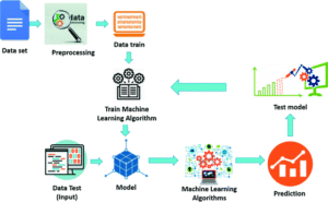
Congratulations for building your very first machine learning model! Its time to understand the essential procedure that data scientists employ across all industries and application. Beginning with data collection and processing to model training evaluating and deployment You now know the whole process.
The foundation allows exploration of more advanced areas like deep learning using neural networks as well as natural language processing reinforcement learning computer vision as well as ensemble techniques. Every project builds your knowledge and knowledge of the best time and what techniques to use.
The field of machine learning is constantly evolving and new frameworks algorithms and the best practices surfacing continuously. Be up to date with online courses as well as research papers Kaggle contests as well as hands on tasks. Join the data science community take part in meetups and work with other people who are facing similar issues.
Keep in mind that even the most experienced data scientists began exactly where you are today. Everyone who is successful in machine learning created a myriad of models made mistakes reconstructed errors and improved through repeated iterations. The first model you build is the start of a thrilling adventure into the world of artificial intelligence and data science.
Keep practicing using a variety of datasets and issues. Develop projects to solve real world issues that you are passionate about. The knowledge youve gained opens the doors to career opportunities in machine learning engineering research in artificial intelligence and business analytics for all industries.
The journey of machine learning is just beginning. Keep building continue to learn increase your knowledge within this exciting area.